Geofenced Searches on Twitter: A Case Study Detailing South Asia’s Covid Crisis
Translations:
Twitter can be a valuable source of information for open source research, both at the level of individual users, but also for understanding broader trends. In a recent Bellingcat story, the Investigative Tech Team looked at patterns in Twitter data to show the severity and speed of escalation of the coronavirus crisis in India.
While Twitter is a common data source for social media analysis because of its public-by-default posting and ease of access for researchers, one limitation is the relative scarcity of geolocation data. Today, very few tweets contain precise geodata, which must be manually added by a user. However, Twitter provides an alternative way to find the location of tweets: geocoded searches.
By using the results of many geocoded queries, Bellingcat was able to make an approximate map of the geographic distribution of tweets looking for urgent assistance across India and its South Asian neighbours, many of which are experiencing their own coronavirus crises. Also mapped is the percentage of these tweets that use the keyword “oxygen,” possibly correlated with medical oxygen shortages.
The method used to collect this data is detailed in the rest of this story, as well as source code that can be adapted for use in other projects. In the process of collecting this data, several peculiarities in Twitter search results were noticed and are also documented below. Because of this, there are some caveats about fine-grained interpretations of this data. Geographic positions are not exact, and the volume of older tweets has been estimated. Estimated data should not be compared directly with non-estimated data. Additionally, as noted in our story in April, English-language Twitter posts are an inherently limited and biased sample given the wide variety of social media platforms and languages used in the region. First though, it’s important to understand how Twitter posts can be found and gathered via location.
Georeferenced Tweets
Some tweets contain precise latitude and longitude information retrievable with the Twitter API. While an API key is necessary to use the Twitter API, this is readily available by applying through the Twitter Developer Portal. However, this only includes geodata that users have explicitly chosen to add to a tweet, and the popularity of this feature has waned. Geocoded searches allow Twitter users to find tweets from within a specified distance of a particular latitude and longitude, and will find tweets that do not contain explicit lat/lng information.
For example, the query ‘geocode:13.08,80.27,100km’ (as shown in the image below) returns tweets that Twitter believes to be from within 100 kilometres of Chennai, India, as specified with the coordinates 13.08º N, 80.27º E. For a full list of Twitter Advanced Search operators, see this document maintained by Igor Brigadir.
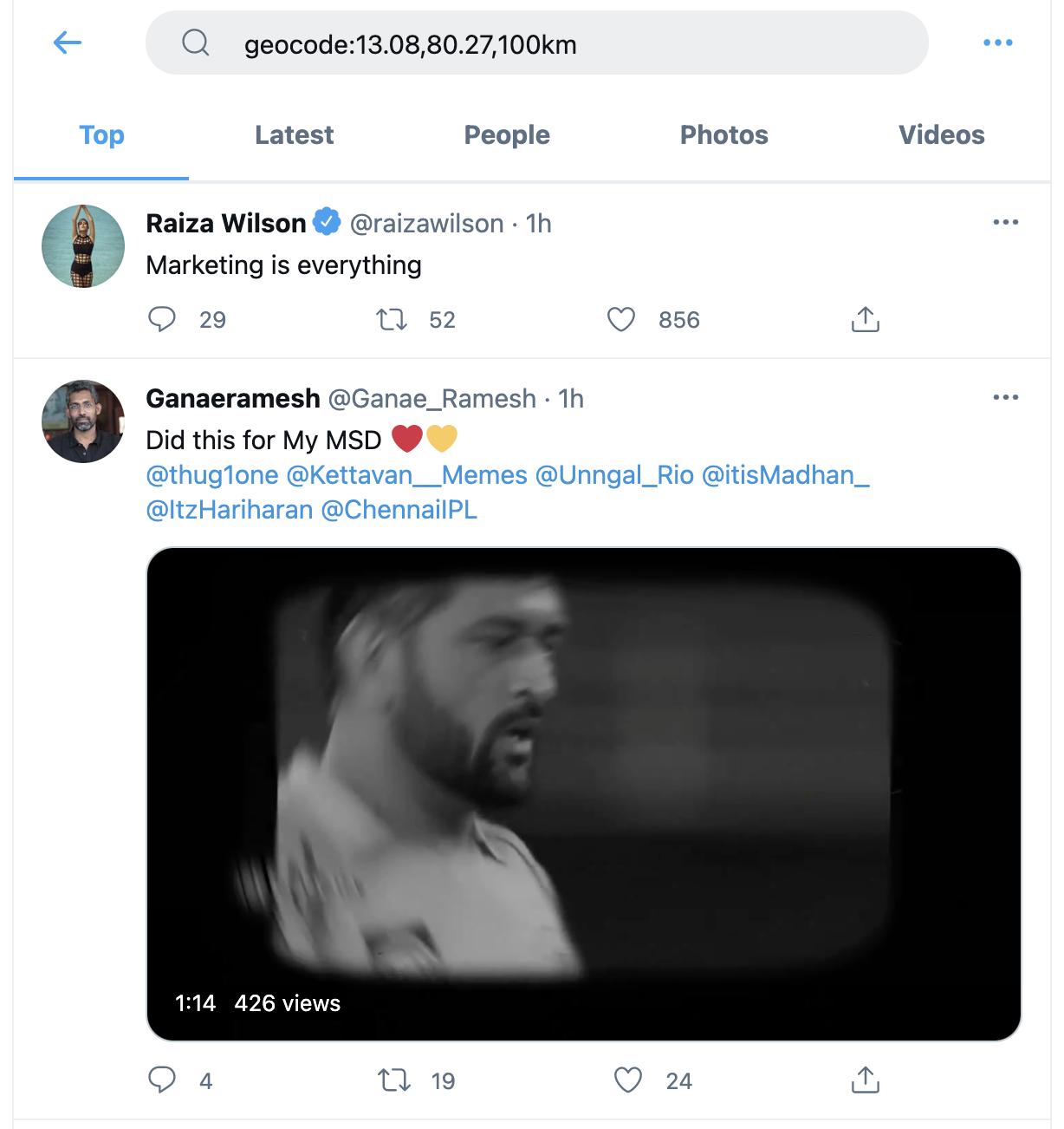
Example search results for a geocoded query.
By using many geocoded queries distributed across an area, a picture of the geographic distribution of a particular topic or situation can be approximated, through both the volume of tweets and the distribution of tweet content. For example, the image below shows the distribution of tweets containing the word “help” or “urgent” on April 25th, 2021, across India and neighbouring regions of South Asia. Each circle is centred at the location of the geotagged query.
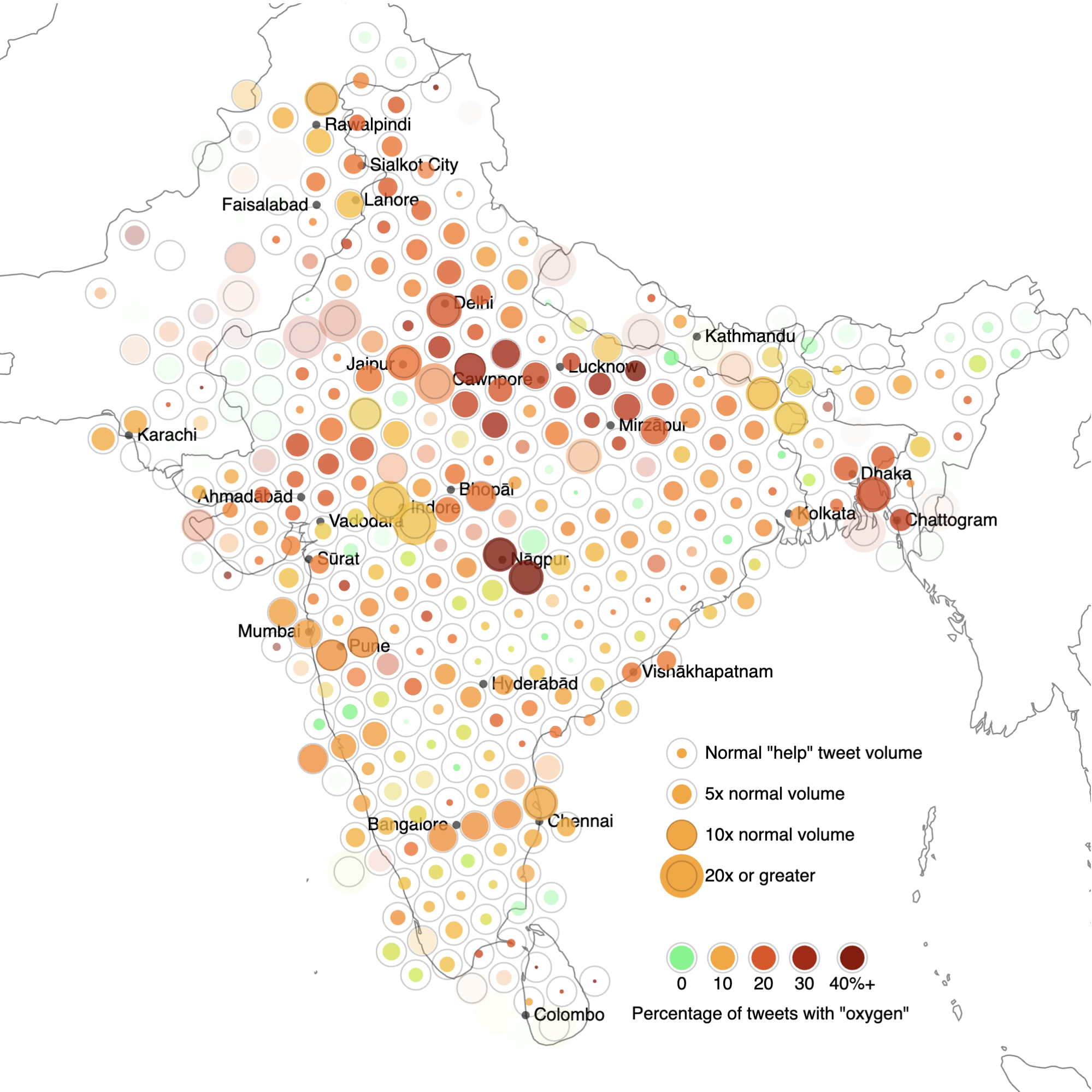
A map showing geotagged posts containing the words “help” or “urgent” across India and neighbouring countries. The colour of each point shows what percentage of these posts also contain the keyword “oxygen.”
This map was created by counting search results for hundreds of geocoded Twitter searches, using TWINT and Python. Thousands, and even millions of tweets can be obtained quickly using TWINT, a useful tool for obtaining Twitter data. TWINT uses the Twitter Advanced Search web interface, and automatically scrapes tweets into a ready-to-analyse format like CSV. See the TWINT Github repository for installation instructions and more examples.
Because TWINT does not use the official Twitter API, it does not require an API key or have rate limitations, which makes it easy to automatically run queries for multiple locations. This methodology, which was also used to create the visualisation at the beginning of this article, is further summarised below. The source code is also provided in a Jupyter notebook, an interactive environment for writing Python scripts.
It is important to first note, though, that this data is only as accurate as Twitter’s own estimation of each tweet’s location. Furthermore, it is not fully transparent how Twitter’s geocode search functionality determines the location to associate with each Tweet. Experimentation and observation by Bellingcat’s Investigative Tech Team found that this data appears to come from two places: tweets which are tagged with a Twitter “place” and the location that a user chooses to add to their Twitter profile. While other sources of geographic information, like user’s IP address or browser tracking data, may be captured by Twitter and used for purposes such as targeted advertising, this information does not appear to be used for georeferenced searches.
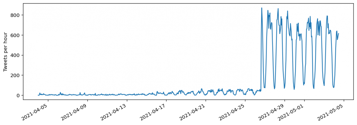
Importantly, user profile location information is only used to georeference tweets for the most recent week (seven to eight days, approximately.) The effect of this is that recent tweet volume appears much greater than that from more than a week ago. While recent tweets contain a mix of both tweets with an explicitly added Twitter “place” tag, and tweets without a place tag, older tweets contain only those with “place” tags.
While the TWINT data is the same as what is manually shown in the Twitter Advanced Search web interface, the official Twitter APIs are slightly different. Bellingcat compared these to each other in order to test variations in Twitter data. There are several different Twitter APIs. We have used both the Standard Twitter API (v1.1), which is free, and the Premium Twitter API, which is paid. The Twitter Premium Search API returns two types of data: individual tweets matching a query, from the “search endpoint”, and counts of the number of tweets that match a query over some time interval, from the “counts endpoint.”
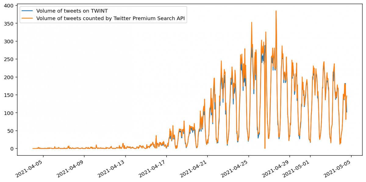
For a simple Twitter search (that is, one without a geocode query), the number of tweets found by TWINT and the Twitter API match quite closely. However, the Twitter Premium Search API counts endpoint does seem to return a slightly greater number of tweets than the TWINT search. This is specified as expected behaviour in the Twitter documentation, as the API may be counting tweets that aren’t visible due to privacy settings or deletions.
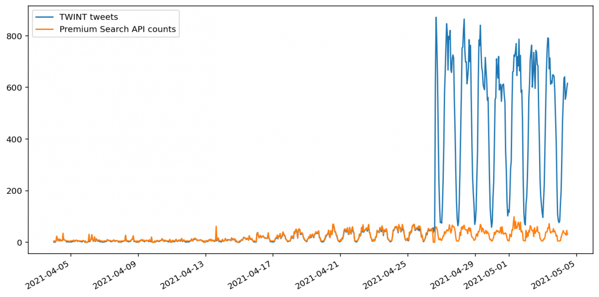
For a geocoded Twitter search, TWINT returns many more tweets for the most recent week, but beyond this time range the quantities closely match. Moreover, all of the tweets returned by the Twitter Premium Search API’s search endpoint are tagged with a Twitter place. This indicates that the Twitter Premium Search API’s geocoding search options do not use Twitter Profile location information, even for recent tweets, unlike the Twitter Advanced Search.
It should be possible to analyse only tweets that have been tagged with a Twitter place, but TWINT’s ability to scrape this data is unfortunately currently broken. This means that there is no way to directly compare older volume with newer volume. A crude multiplicative correction is demonstrated in the data visualisation Jupyter notebook, but this should be understood to be very approximate.
Also of note here is that the Twitter Premium API counts endpoint appears to round up any value between one and five tweets to five. Zero appears to be retained as zero.
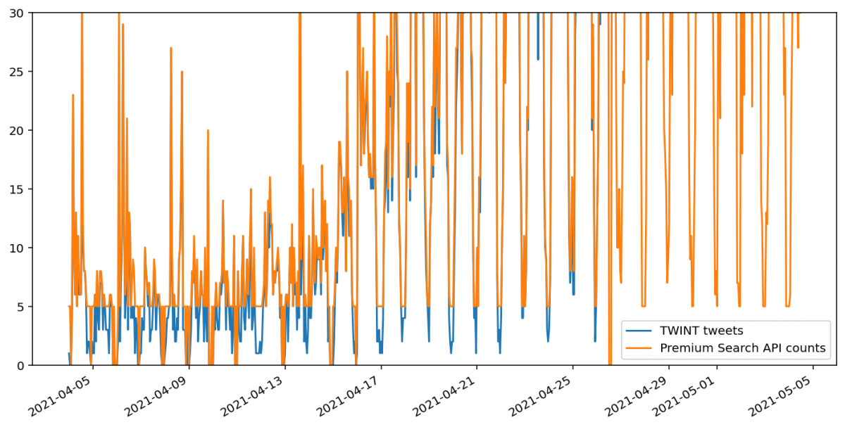
While this behaviour for the most recent week matched the tweets returned by the Premium Search API search endpoint, it does not match the Standard Twitter API’s search endpoint. Instead, tweet counts via this endpoint are close to those returned by TWINT. However, some do appear to be missing.
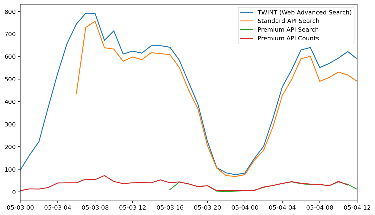
Tweets per hour for the same geocoded search using several different methods to obtain tweet data. The standard Twitter API search more closely matches the results returned by TWINT.
A cursory inspection of tweets that were captured by TWINT but not the Standard API did not reveal any obvious reason why they were excluded. In this case, not only was TWINT easier to use, it appears to retrieve more complete datasets.
Code and data detailing these observations is available in a Jupyter notebook.
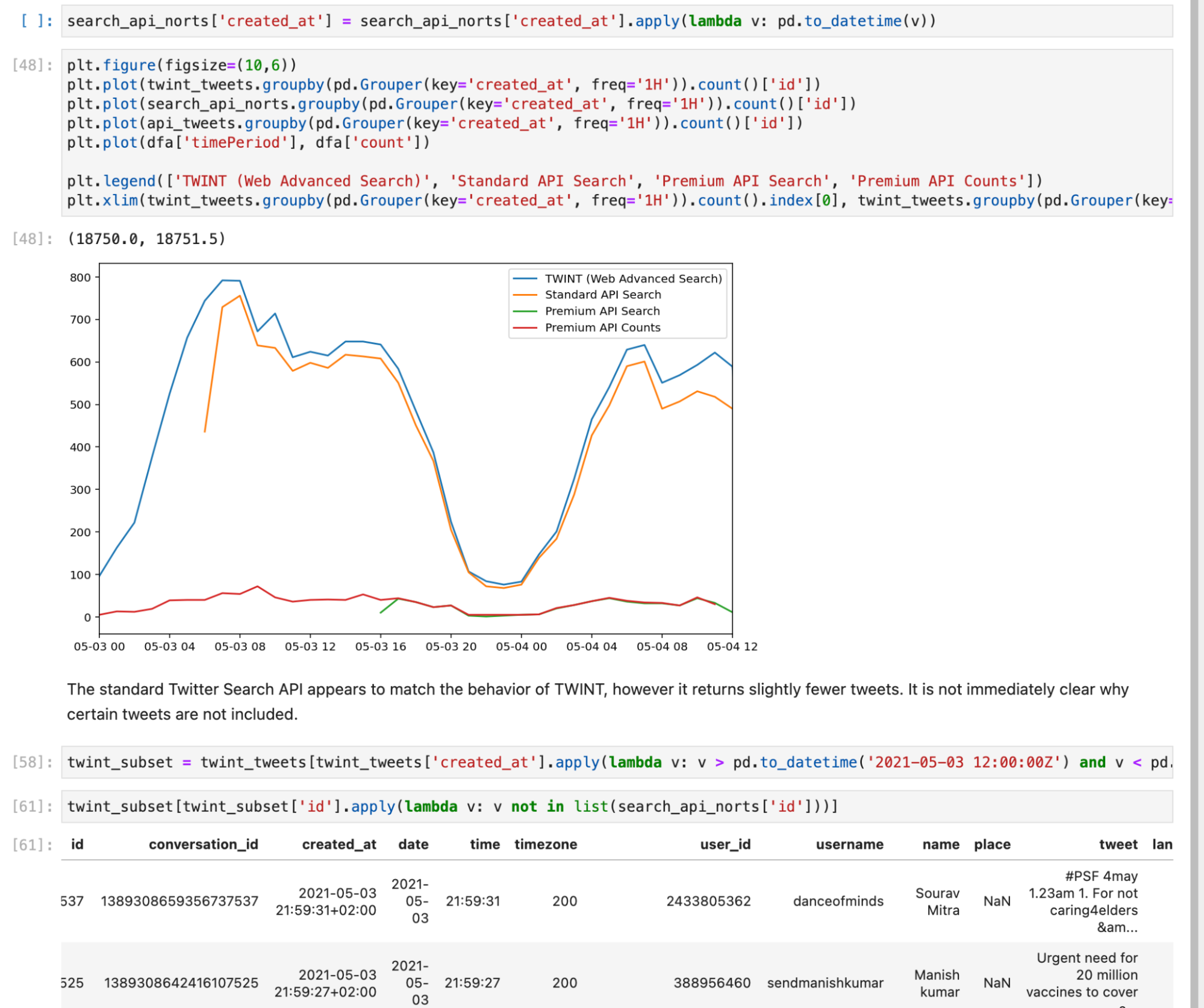
A screenshot from the Jupyter notebook showing how data was obtained and analyzed. This open source notebook allows Bellingcat’s observations to be replicated independently.
Building a Map of Tweet and Term Frequency
In order to use Twitter geocode search functionality to build a map of tweet frequency, a hexagonal grid of center points is needed. Hexagonal packing is the best way to cover the entire area with the smallest amount of overlap between adjacent circles.
While many libraries exist to generate hexagonal tilings, for this project Uber’s H3 library was used. It has some nice properties, including spherical tiling and approximately equally sized tiles. The H3 Python libraries contain methods for finding all tiles that have a centre within a particular polygon. For this example, a rough outline of India and its South Asian neighbours was used.
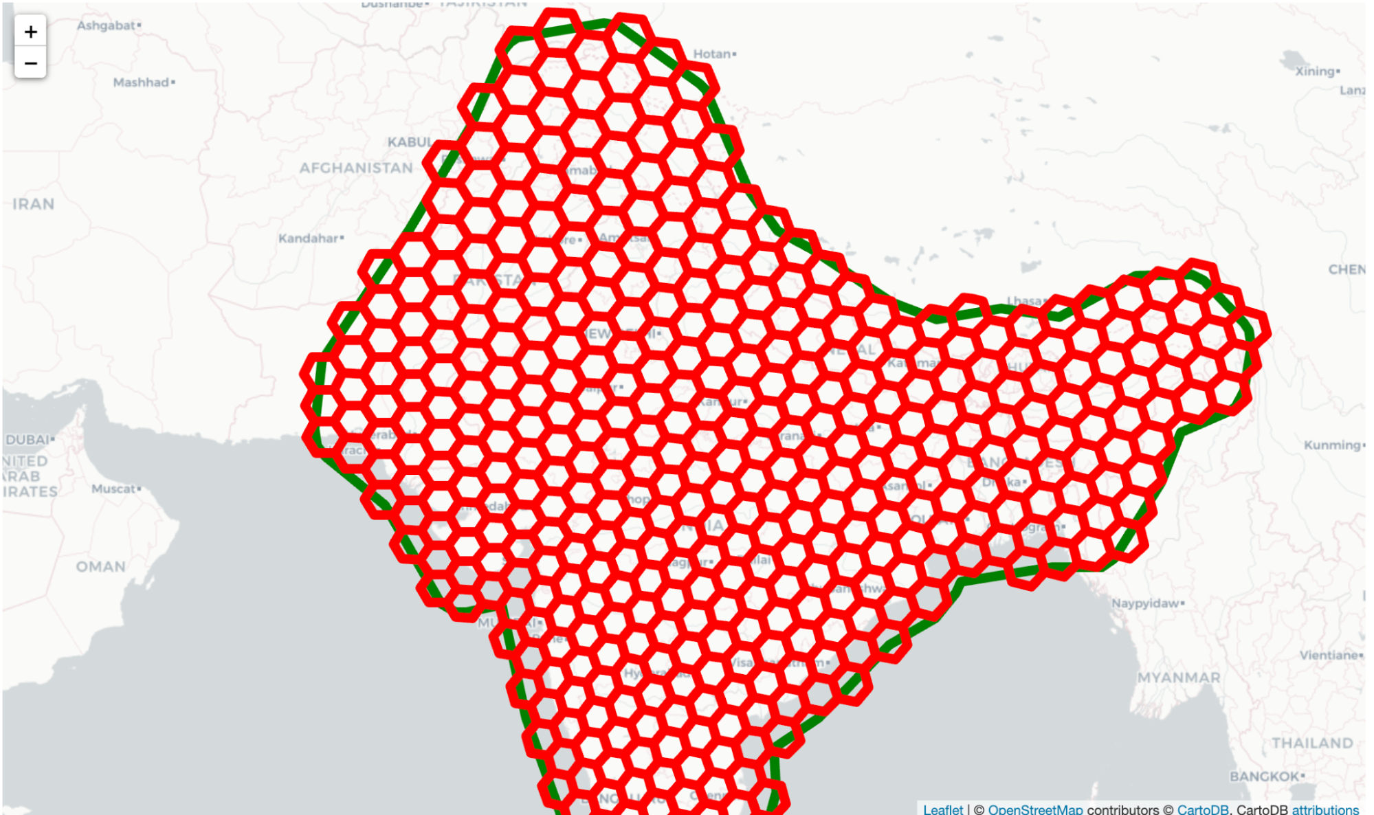
A map of H3 tiles that fall within a particular area of interest (in this case, India and its neighbours, indicated by the thick green line.)
However, since Twitter only allows circular queries via the Advanced Search, these hexagons must be converted into overlapping circles. Using the area of each tile, also available conveniently via H3, a radius was computed for a circle that would approximately cover it. Each tile radius and centre was used to create a custom search query for each cell. For example, “(urgent OR help) AND geocode:22.089682313298564,81.20150766588854,69.85968148546738km”. Because each circle contains the entire hexagonal cell, there will be some overlap of search queries near cell edges. This results in a small loss of geographic accuracy, however, this is a much smaller concern than the inherent limitations in Twitter’s location accuracy to begin with.
Next, TWINT was used to download the search results for each cell’s search query, and the Python data analysis library “pandas” was used to group each of those tweets by day and count the volume. Since some cells have a much greater population than others, each cell is normalised by calculating a baseline/normal tweet volume, which is simplistically the average across the entire time range.
This Jupyter notebook contains source code that shows how this is done in more detail, and how to export the data as CSV files that can be used for further visualisation.
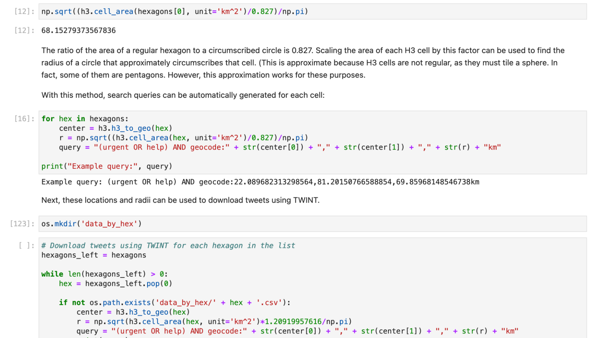
A screenshot from a Jupyter notebook showing how this technique of repeated geocode queries was used to build data for the visualisation.
As discussed and demonstrated earlier, there is a difference in how tweets from the most recent week are treated by the Twitter Advanced Search. The results in an artificial jump in a timeseries of the number of tweets posted per day. There is no straightforward way to compensate for this. While searches with the official Twitter Search API return more consistent data (albeit with a smaller number of tweets), they do not support a geographic radius greater than 40 km.
As an approximate compensation, Bellingcat used the volume differences between searches at different points in time to estimate the ratio of tweets “missing” after a week. This is essentially an estimate of the percentage of users that have a valid location in their profile description as compared to users that use location tags. This corrective multiplicative factor produces volume estimates that are closer to the range of the most recent week. However, the variance of this factor was very large, as it heavily depends on the posting patterns of users in a particular geographic area. This multiplicative correction should be considered a very approximate estimate at best. As a result, “estimated” figures cannot be compared directly with the more recent figures.
However (to the extent that each sample is random), trends in tweet content such as the percentage of tweets containing a certain keyword, can still be compared across this time boundary. This allows an examination of how tweets for oxygen related needs spread across India from Delhi, both as other cities were besieged and as Twitter users from other places and countries amplified Delhi’s pleas. Tweets from neighbouring countries mention oxygen less frequently.
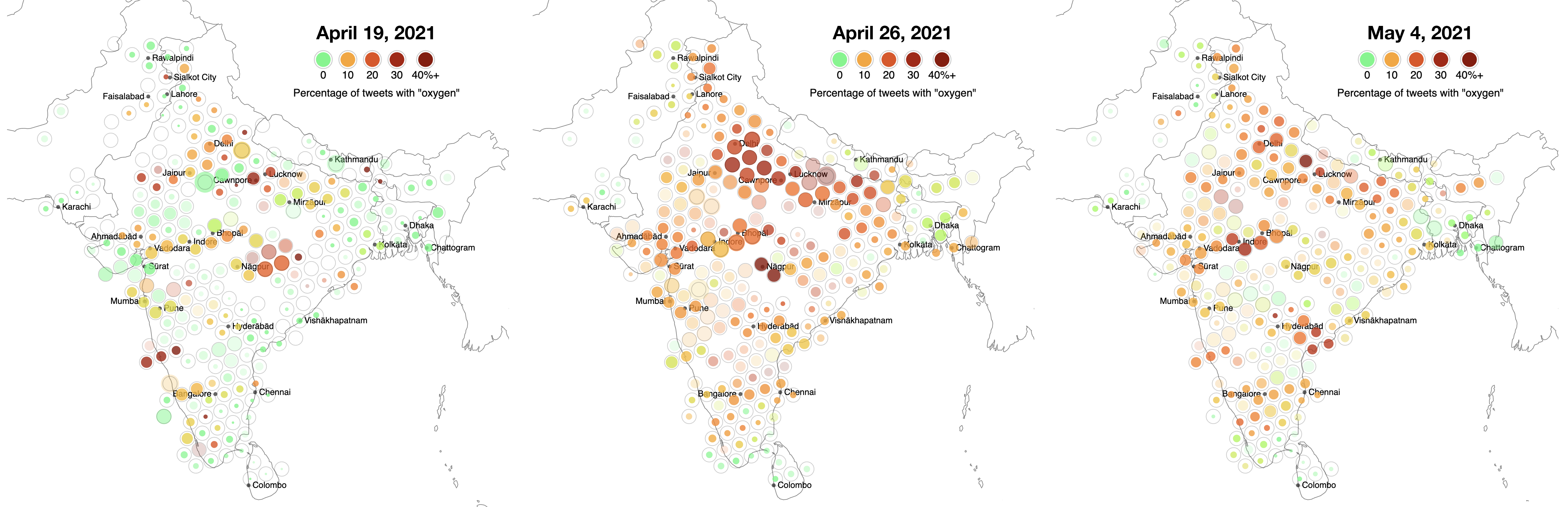
Color indicates the ratio of urgent tweets containing oxygen-related keywords. Left: data from April 19th, 2021, shows hot spots near Lucknow and Kanpur, and a growing crisis in Delhi. Center: On April 26th, the crisis intensified in Delhi. Many other parts of India also saw a dramatic rise in oxygen related tweets, possibly as a result of local crises, and possibly as a result of amplification of the situation in Delhi. Right: by May 4th, 2021, tweets about the oxygen crisis in Delhi had abated to some extent. However, some hotspots, such as around Indore, are still visible. Click or tap to enlarge image.
Despite the limitations imposed by the Twitter API, it is possible to extract geographic information from tweets. While this data comes with many caveats about accuracy and sample bias, it is nonetheless an interesting resource for tracking global events via social media.
The Bellingcat Investigative Tech Team develops tools for open source investigations and explores tech-focused research techniques. It consists of Johanna Wild, Aiganysh Aidarbekova and Logan Williams. Do you have a question about applying these methods or tools to your own research, or an interest in collaborating? Contact us here.